# 3.0 Advanced Dashboard Primer

Aren't you an intrepid explorer! Look at you jumping right to the advanced section! Well, we are glad you are here. In this section we'll be looking at how you can create much more complex dashboard content.  
  
As soon as you want to go beyond supplied panels, or direct data from inventory queries, then things are going to get a bit more complex. However, don't be daunted! We are going to give you the building blocks here for building complex and very meaningful aggregate data from FileWave sources.  
  
Please see the articles below for the elements we'll build on:

# 3.1 Aggregating Data

## What

The FileWave dashboard can show raw device data, but aggregated data is what gives you the quick summary. Aggregation rolls many records into something easier to read, such as counts by version, model, or status.

## When/Why

Use aggregation when you need the big picture instead of a long list. For example, if you are rolling Java from build 183 to build 196, a per-device report shows every record, but an aggregated view shows how many devices are still on each version. That makes rollout progress much easier to understand at a glance.

## How

To get aggregated data into Grafana, create a Prometheus scrape job that summarizes the inventory-query data you care about. The next articles in this section walk through that process: define the Prometheus job, test the scrape, review the resulting metric in Explore, and then turn it into a panel.

# 3.1.1 Grouping Data Using Prometheus

## What

In order to do summary reporting, we need to leverage the power of Prometheus.

## When/Why

Anytime we want to do something like report on a rollout or general status, we are going to want to summarize a report. We will accomplish this by using a Prometheus config file on the FileWave server itself.

## How

The configuration (or yml files) that we'll create will always be placed in the **/usr/local/etc/filewave/prometheus/conf.d/jobs/https** directory on the FileWave server. Anything placed in this directory will automatically be read by Prometheus, and the data presented to our dashboard. (Example yml files can be found in /usr/local/etc/filewave/prometheus/conf.d/jobs)

The syntax of these files is quite picky, so it is best to copy an existing one, and then modify it. It may seem complicated, but we are always going to do the following steps:

<table id="bkmrk-%C2%A0-%C2%A0-step-example-1.-"><thead><tr><th> </th><th> </th></tr></thead><tbody><tr><td>Step</td><td>Example</td></tr><tr><td>1. Place a new (or copied) yml file into /usr/local/etc/filewave/prometheus/conf.d/jobs/https with a meaningful name.</td><td>![image2020-8-11_13-31-54.png](https://kb.filewave.com/uploads/images/gallery/2023-07/e4kS94SKs3qxXpmV-image2020-8-11-13-31-54.png)</td></tr><tr><td>
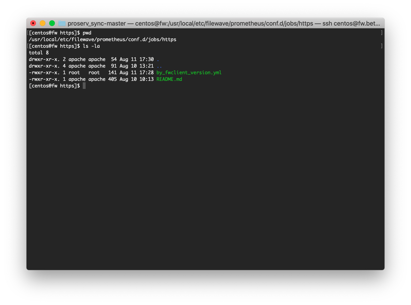
2. Edit the new file to specify the following 3 things:  
  
\* The inventory query (report) to use  
\* The field you want to count by...device\_id is almost always a good one if reporting by device  
\* The field you want summarize (aggregate) by...in this case, the filewave client version</td><td> </td></tr><tr><td>3. Once your report is created, the report id to use is most easily accessed through the webadmin. Note that the fields you want to use for aggregation must be in the report.</td><td>![Report YML Config.png](https://kb.filewave.com/uploads/images/gallery/2023-07/F35g36Iot5EL6xEh-report-yml-config.png)</td></tr><tr><td>
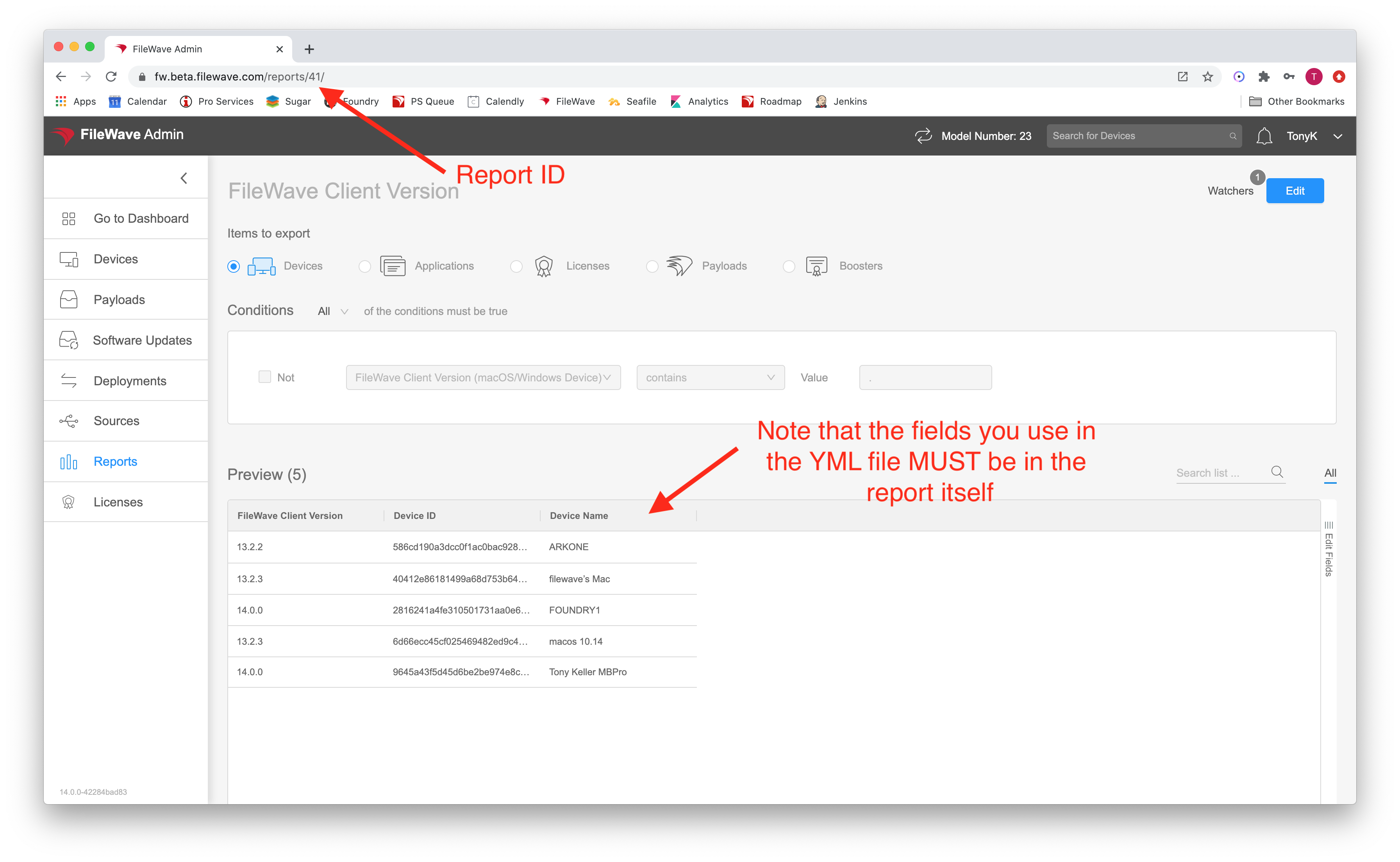
4. Get the definition for the fields you want to use from the API...the easiest way is to do a curl from the command line like this:   
  
`bash<br>curl -s -k -H "Authorization: <Base64_API_Token>" https://<my.server.address>:20445/inv/api/v1/query/<report_id> | python -mjson.tool<br>`  
  
Make sure and substitute in your values for the &lt;Base64\_API\_Token&gt;, &lt;my.server.address&gt; and &lt;report\_id&gt;  
  
You'll get a response that includes the component and the field names as shown at right</td><td>![image2020-8-11_14-43-10.png](https://kb.filewave.com/uploads/images/gallery/2023-07/cigapWuESXaaVaFj-image2020-8-11-14-43-10.png)</td></tr><tr><td>
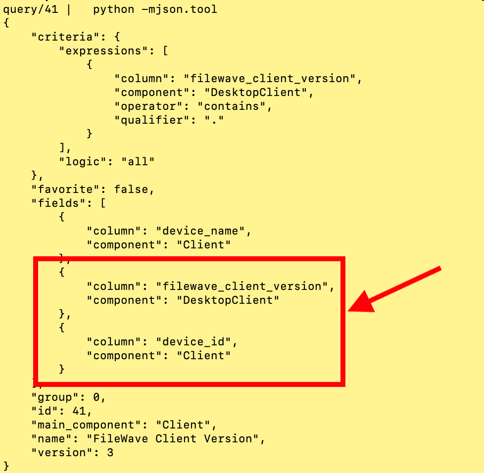
4. Edit the YML file to specify the 3 items as they match your report definition, then save the file. If using the sample file, remember to take out the comment # at the beginning of each line. Example at right:</td><td>![image2020-8-11_14-50-19.png](https://kb.filewave.com/uploads/images/gallery/2023-07/yJhig0WZ1YeFgvDx-image2020-8-11-14-50-19.png)</td></tr></tbody></table>

Within a minute or two of creation of the file, the data should be available in your dashboard for a new panel.

# 3.1.2 Testing the Prometheus Scrape

## What

Assume for a moment you made a typo in the yml file, or some other problem occurs and your new scrape isn't showing in Grafana...how can you see what is going on?

## When/Why

Thankfully there is a service running that allows you to see the status of all Prometheus scrapes, and will usually give you an idea about what is going on. We can check a web page to get this detailed information.

## How

The webpage/port in question though is NOT open by default to external systems and we must access it in a special way. If the port were open, we would normally just go to [https://my.server.address:21090/targets](https://my.server.address:21090/targets,). But, to work around the port not being opened, we can do the following (from terminal, macOS):

<table id="bkmrk-ssh--l-8000%3Alocalhos"><tbody><tr><td>
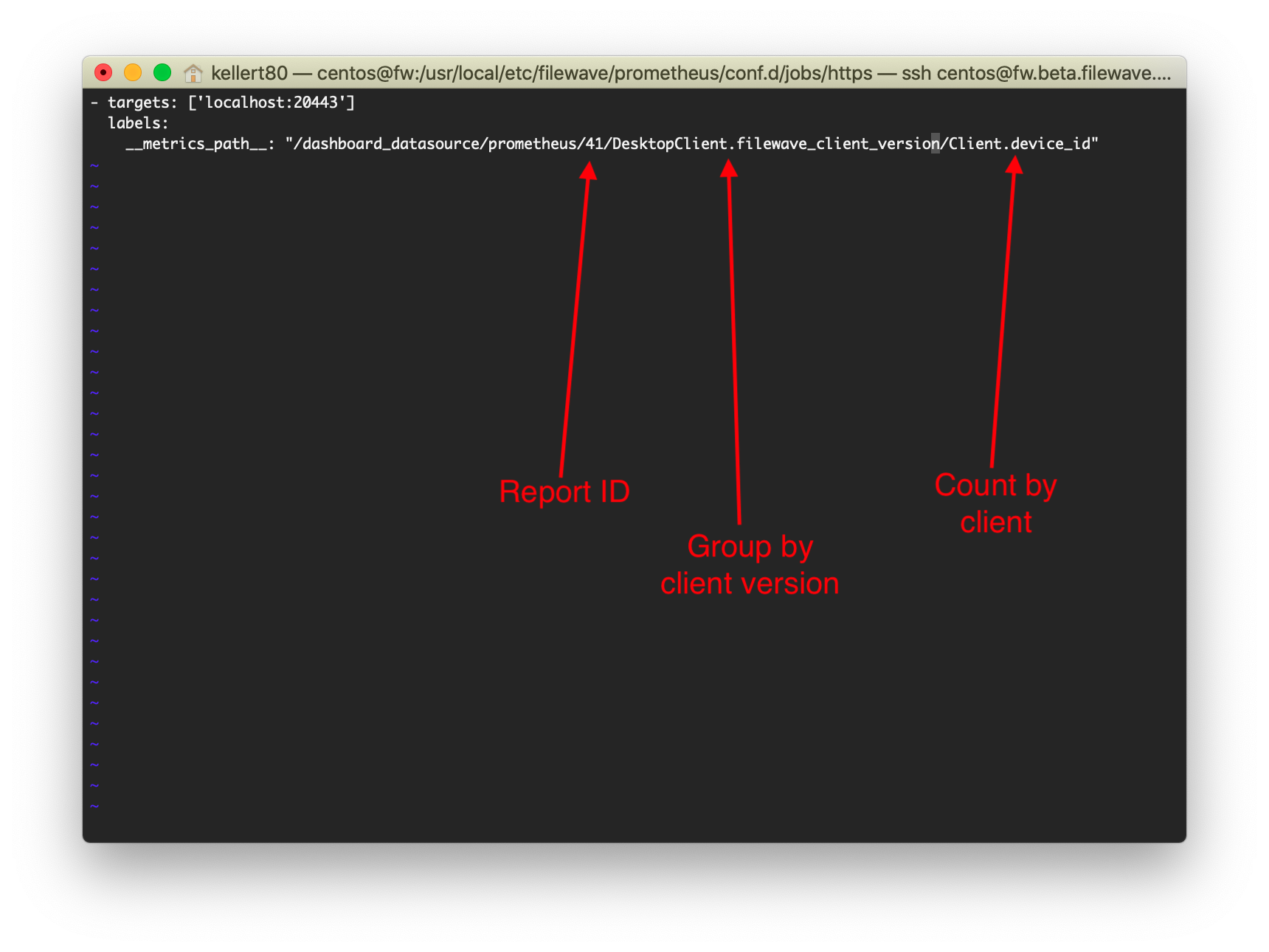
ssh -L 8000:localhost:21090 user@my.server.address

</td></tr></tbody></table>

Alternatively, if you are on a Windows device, you can do the same thing through Putty by configuring a "tunnel" with local port of your choosing redirecting to the FileWave server:

![](https://kb.filewave.com/uploads/images/gallery/2023-07/K4MSsRmyL9adviPm-embedded-image-iyskfedd.png)

These configurations redirects our requested traffic back to port 8000 on our local device, based on the ssh connection being established. The result is that in our own browser then, we can go to [http://localhost:8000/targets](http://localhost:8000/targets) to see the scrape data.

See below how I have a mistake in one of my jobs (query 153 doesn't actually exist):

![](https://kb.filewave.com/uploads/images/gallery/2023-07/pidPLTTtnN4iQpYz-embedded-image-q0djazlc.png)

# 3.1.3 "Exploring" Your New Aggregate Data

## What

Before you build a formal Grafana panel, it often helps to look at the aggregated data directly. The Explore view is the fastest way to sanity-check what your report is producing.

## When/Why

Use Explore after you have configured the Prometheus scrape and want to confirm the metric looks right before turning it into a panel.

## How

Aggregated inventory-query data is exposed in Dashboard metrics as `filewave_inventory_query_<id>`, where `<id>` is the report ID you used. The attached video shows the Explore workflow for one of those metrics.

<video controls="" height="300" poster="" width="600"><source src="https://kb.filewave.com/attachments/61"></source></video>

In this example, the data is no longer shown as five separate records. Instead, it has been grouped into three records because only three different FileWave client versions are present across the endpoints. That grouped result is much easier to use when you build a chart, such as a pie chart, in the next step.

# 3.1.4 Creating your Data Panel

## What

Once your aggregated metric is available in Grafana, you can turn it into a panel that answers the question you actually care about.

## When/Why

Pick the visualization based on the story the data needs to tell. Pie charts work well for a current distribution, such as how many devices are on each client version right now. Line or bar charts are better when you want to watch that same data change over time.

## How

Creating the panel is similar to the earlier dashboard examples, but now you are working with aggregated Prometheus data instead of a simple raw query result. The video below shows the basic workflow.

<video controls="" height="300" width="600"><source src="https://kb.filewave.com/attachments/62"></source></video>

Grafana gives you a lot of freedom in how a panel is presented. One small detail that helps immediately is the legend format. In this example, using `{{genericdesktopclient__filewave_client_version}}` makes the legend display the actual version value instead of a less useful raw field name.

We chose **Instant** in this example because the goal is a current snapshot, which is usually the right choice for a pie chart. If you want to see the same metric trend over time, use a visualization such as a bar or line chart and query the time-series data instead.

# 3.2 Extra Metrics

## What

We learned in the 3.1 section how to build our own custom panels. "Extra Metrics" is an independently built tool to automate creation of a few reporting elements for us without doing it manually. This solution is NOT directly supported by FileWave, but you may find it useful in your environment.

## When/Why

"Extra Metrics" gives data on applications, and generally on patch status of your devices. The patch status elements are hard-coded, but the application versions panels are driven by dynamic reports that you can tweak to fit your needs. All information for installation and upgrade of this solution is found here: [https://pypi.org/project/filewave-extra-metrics/#description](https://pypi.org/project/filewave-extra-metrics/#description)

## How

In this example, we have Extra Metrics installed, and are adding a new report to view Firefox information on macOS devices.

<video controls="controls" height="300" width="600"><source src="https://kb.filewave.com/attachments/63"></source></video>